
Complex Network Analysis of MCI and AD Patients
Alireza Fathian |November, 2020
1. Introduction
By creating networks that model the functional brain connectivity of different subjects, we have shown that there are topological differences between subjects of each group.
2. Methods
2.1. Subjects
The rs-fMRI and T1w images of 92 subjects from ADNI database were analyzed in this study.
| CN | EMCI | LMCI | AD | ALL | |
|---|---|---|---|---|---|
| Sample Size | 23 08 M 15 F |
23 12 M 11 F |
23 10 M 13 F |
23 11 M 12 F |
92 41 M 51 F |
| Age (Mean±SD) |
75.82±9.44 | 75.29±6.36 | 72.26±7.05 | 77.75±3.75 | 74.78±7.11 |
2.2 Preprocessing
Preprocessing data was done using fMRIPrep. fMRIPrep is a fMRI data preprocessing pipeline that performs basic processing steps on raw images. Including:

2.3. Denoising
A selection of nuisance variables generated by fMRIPrep were regressed out of the data. These variables are:
- 6 motion estimates
- Mean signal in WM, Mean signal in CSF
- Global signal regression
In addition to that, the derivatives, quadratic terms, and squares of derivatives of these variables were also regressed out.
2.4. Parcellation
In this step, the brain were parcellated into 360 regions by the HCP-MMP parcellation. The time series corresponding to each region were computed as the mean of time series of voxels within that region.
2.4. Parcellation
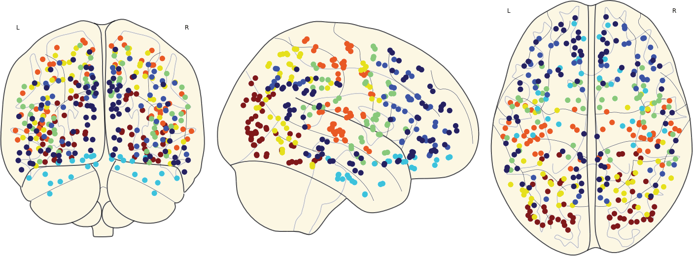
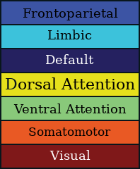
| Visual | Somatomotor | Limbic | Default |
| DorsalAttention | VentralAttention | Frontoparietal |
2.5. Correlation Matrix
The correlation among time series corresponding to different brain regions were computed with two different methods, Pearson's correlation coefficient and GLASSO. These correlations then were used to create undirected networks of functional connectivity.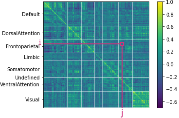
The element within represents the correlation between nodes $i$ and $j$.
2.6. Adjacency Matrix
Adjacency matrices were created by thresholding the correlation matrices. we have choosed the thresholding values that maximizes the global cost efficiency (GCE). \begin{aligned} Threshold & = \underset{-1 \leq t\leq 1}{\mathrm{argmax}}(GCE(t)) = \underset{-1 \leq t\leq 1}{\mathrm{argmax}}(E(t) - PSW(t)) \end{aligned} \begin{aligned} E(t) & = \frac{1}{n}\sum_{i\in N}^{}\frac{\sum_{j\in N,j\neq i}^{ }(\frac{1}{d_{ij}})}{n-1}, PSW(t) = \frac{\sum_{i\in W,i\geq t}^{}i}{\sum_{j\in W}^{}j} \end{aligned}where $E$ is the global efficiency, $PSW$ is the proportion of the strong weights, $N$ is the set of all nodes, $n$ is the number of nodes, $d_{ij}$ is the shortest path length between nodes $i$ and $j$, and $W$ is the set of all weights
2.7. Network Measures
For each network 10 local and 14 global network measures were computed:
- Local Measures: Density, Average Shortest Path Length, Transitivity, Average Clustering, Local Efficiency, Global Efficiency, Pearson Correlation, Degree Assortativity Coefficient, Diameter, Radius.
- Global Measures: Degree, Eccentricity, Betweenness, Communicability Betweenness, Eigenvector, Katz, Closeness, Current Flow Closeness, Load, Clustering Coefficient, Pagerank, Subgraph, Harmonic, Strength.
2.7. Network Measures
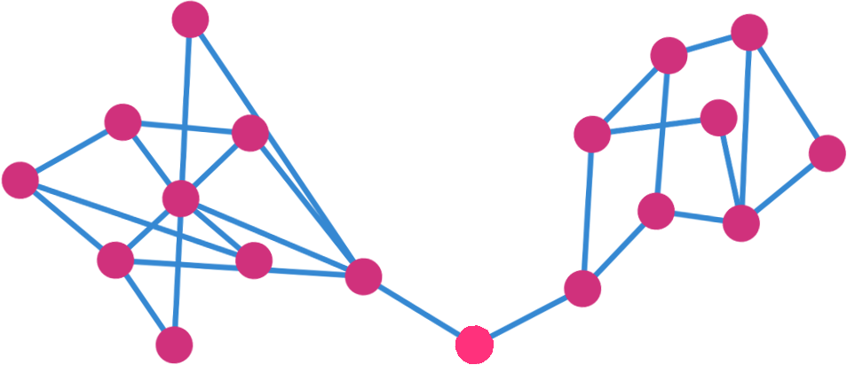
- Clustering
- Betweenness Measure of the influence of a vertex over the flow of information between every pair of vertices.
Clustering measures the tendency of neighbors of a node to be also neighbors.

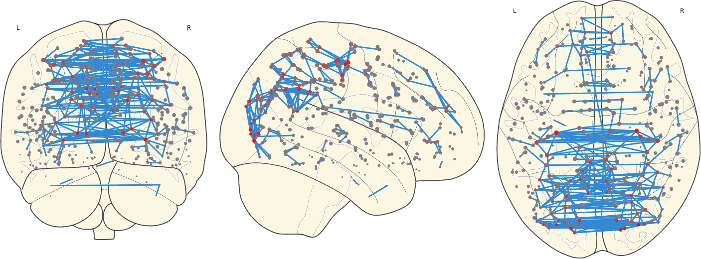
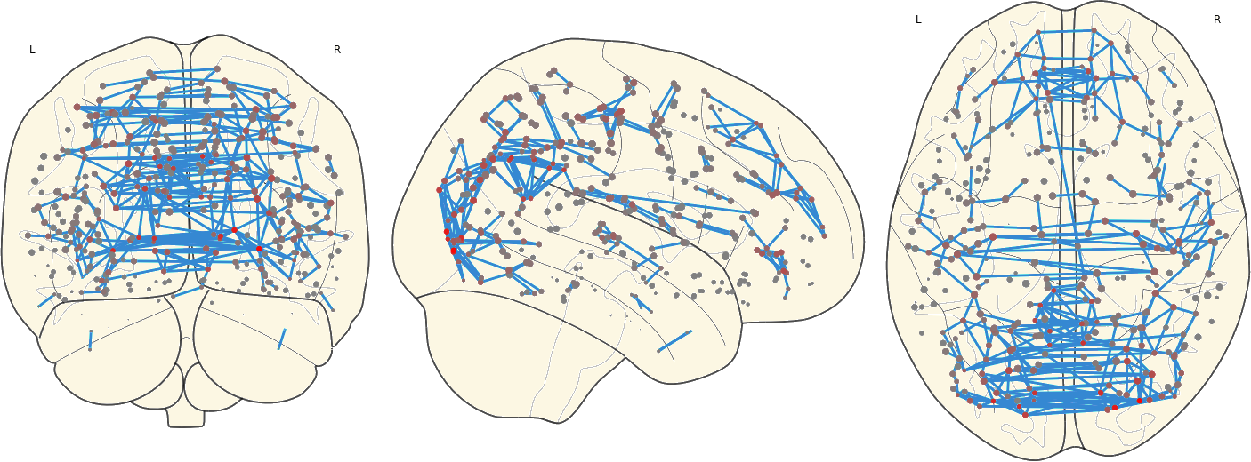
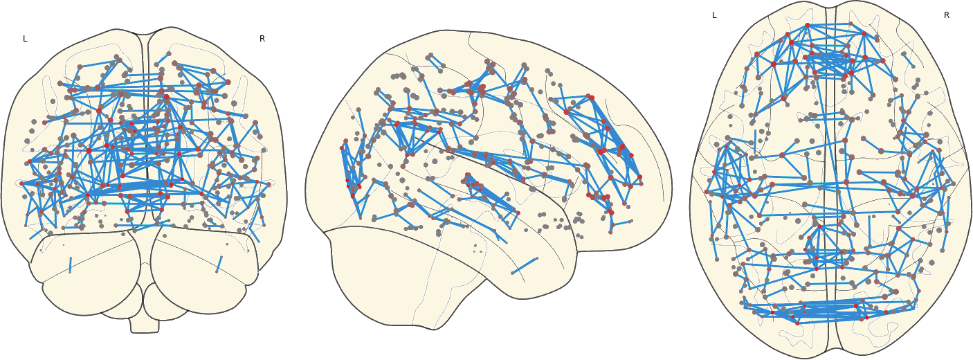
2.8. Mean Network
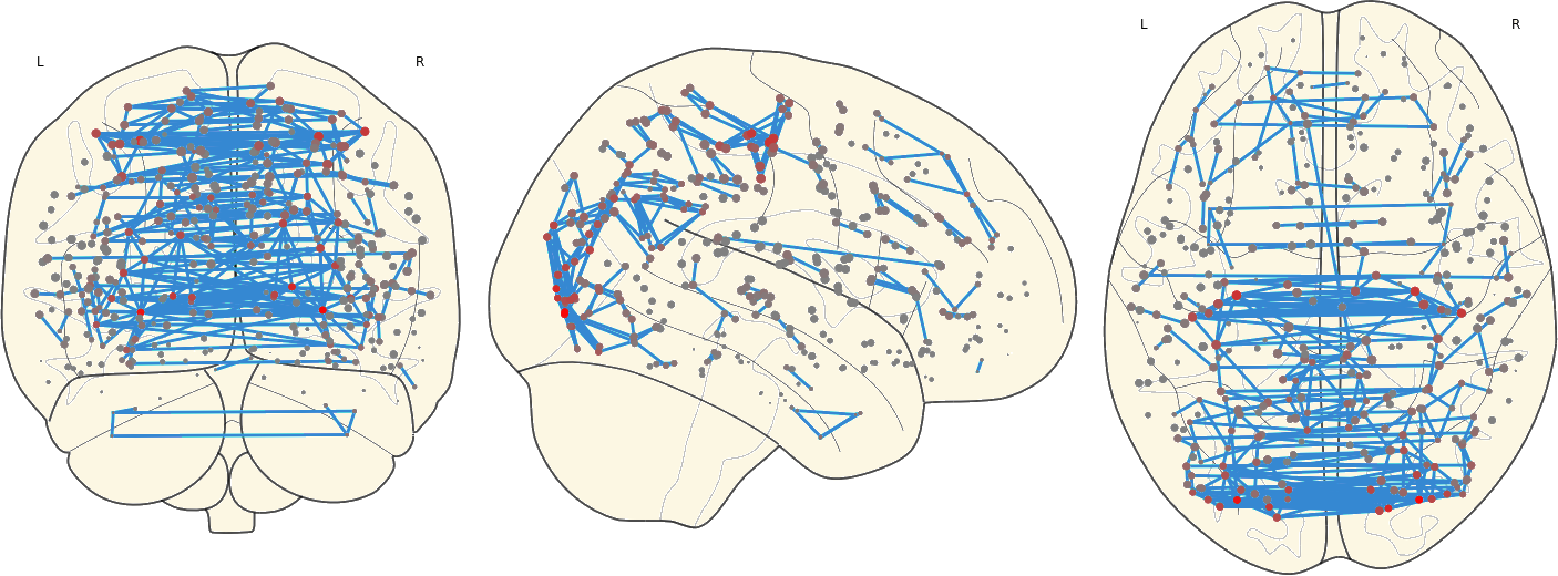
For each subject in a group the mean network were computed as the voxel-wise mean of all subjects within that group.
2.8. Mean Network
2.8. Mean Network
2.8. Mean Network
2.8. Mean Network
3. Results
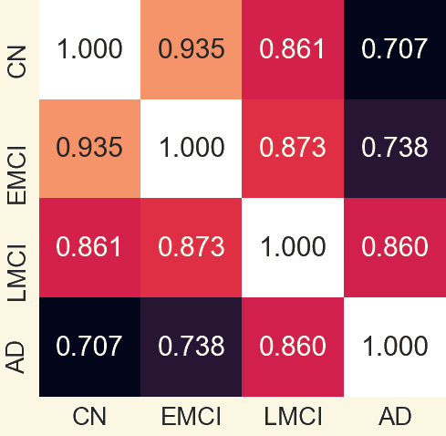
3.1 Pearson Correlation Coefficient Among Mean Networks
3.1 Pearson Correlation Coefficient Among Mean Networks
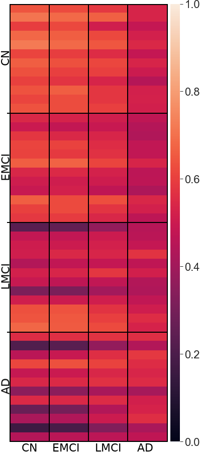
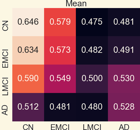
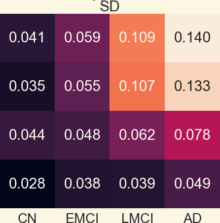
3.2 Analyzing Measures: Global Measures of Mean Networks

3.2 Analyzing Measures: local Measures of Mean Networks
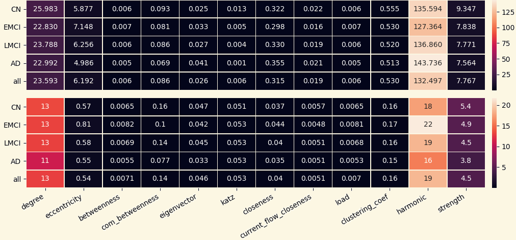
3.2 Analyzing Measures: Histogram of Strength
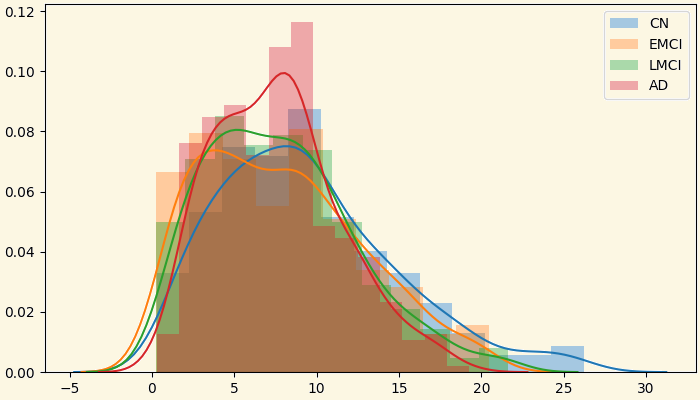
3.3 Analyzing Measures: Relationship Between Groups Based on Measures

Strength Clustering Betweenness Closeness
3.3 Analyzing Measures: Relationship Between Groups Based on Measures

Strength Clustering Betweenness Closeness
3.3 Analyzing Measures: Relationship Between Groups Based on Measures

Strength Clustering Betweenness Closeness
3.3 Analyzing Measures: Relationship Between Groups Based on Measures

Strength Clustering Betweenness Closeness
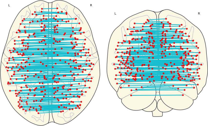
3.4 Symmetric Links
The mean of the correlation coefficients of pairs of nodes that are symmetrical to each other.
Group |
Mean |
SD |
|---|---|---|
| CN | 0.708 | 0.060 |
| EMCI | 0.696 | 0.073 |
| LMCI | 0.613 | 0.148 |
| AD | 0.533 | 0.154 |
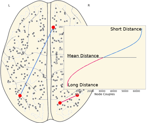
3.5 Long and Short Links
We have classified links as short and long links based on the spatial location of its nodes on the brain.
| Short Links | Long Links | |||
|---|---|---|---|---|
Group |
Mean |
SD |
Mean |
SD |
| CN | 1.128 | 1.896 | 0.441 | 1.309 |
| EMCI | 1.114 | 1.950 | 0.454 | 1.360 |
| LMCI | 1.114 | 1.915 | 0.455 | 1.340 |
| AD | 1.065 | 1.910 | 0.501 | 1.403 |
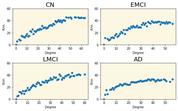
3.6 Assortativity
The tendency of nodes to connect to other nodes with similar degree.
Measuring Assortativity: The average nearest neighbors degree of a vertex $i_{k}$: \begin{aligned} k_{nn,i} & = \frac{1}{k_{i}}\sum_{j\in V(i)}^{}k_{j} \end{aligned} The average degree of the nearest neighbors, $k_{nn}(k)$, for vertices of degree $k$: \begin{aligned} k_{nn}(k) & = \frac{1}{N_{k}}\sum_{i/k_{i}=k}^{}k_{nn,i} \end{aligned} Where $k_{i}$ is the degree of node $i$, $V(i)$ is the set of neighbours of node $i$, and $N_{k}$ is the number of nodes with degree $k$.3.6 Assortativity
Group |
Pearson assortativity coefficient |
|---|---|
| CN | 0.708 |
| EMCI | 0.696 |
| LMCI | 0.613 |
| AD | 0.533 |
3.7 CL(k)-Knn Plot
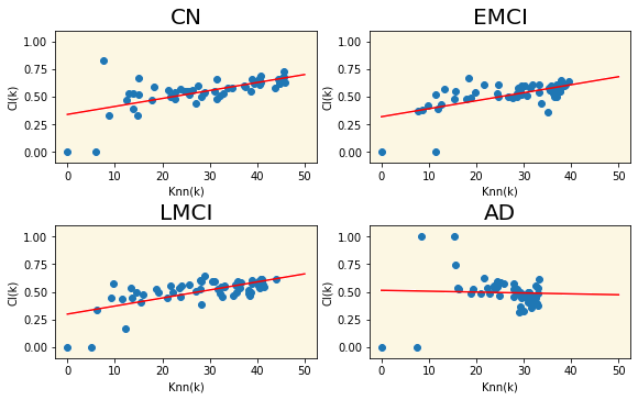
Group |
Slope of the fitted line |
|---|---|
| CN | 0.00723 |
| EMCI | 0.00726 |
| LMCI | 0.00729 |
| AD | -0.00080 |
3.8 Rich-Club
Rich-club measures the tendency of high degree nodes, to be connected to each other, forming subgraphs more easily than low degree nodes. \begin{aligned} \phi(k) = \frac{2 E_{>k}}{N_{>k}(N_{>k}-1)}, \rho_{ran}(k)=\frac{\phi(k)}{\phi_{ran}(k)}, \scriptscriptstyle where \begin{gather} E_{>k}\, is\, the\, number\, of\, edges\, among\, the\, N>k\, nodes \\ N_{>k}\, is\, the\, number\, of\, vertices\, with\, degree\, larger\, than\, k \end{gather} \end{aligned}
3.9 Small-world Property
A network has a small-world property if it is possible to go from one vertex to any other in the network passing through a very small number of intermediate vertices.
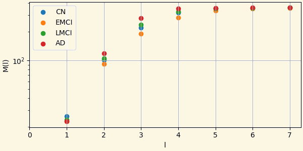
$M(l)$ the average number of nodes within a distance less than or equal to from any given vertex.
In small-world networks this quantity follows an exponential or faster increase.
3.10 Classifying Nodes
We have classified nodes into 7 modules based on the 7-ROI parcellation by Yeo et al., (2011).
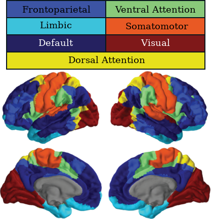
| weights of inter-ROI links |
weights of intera-ROI links |
|||
|---|---|---|---|---|
Group |
Mean |
SD |
Mean |
SD |
| CN | 0.197 | 0.171 | 0.003 | 0.120 |
| EMCI | 0.182 | 0.155 | 0.007 | 0.107 |
| LMCI | 0.173 | 0.156 | 0.012 | 0.114 |
| AD | 0.153 | 0.166 | 0.014 | 0.128 |
3.10 Classifying Nodes
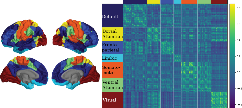
CN EMCI LMCI AD
3.10 Classifying Nodes
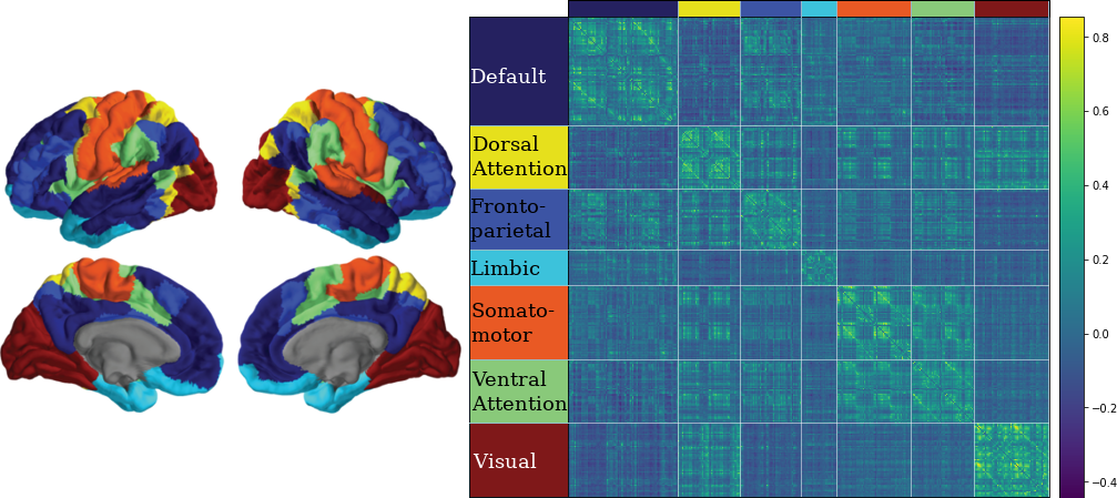
CN EMCI LMCI AD
3.10 Classifying Nodes
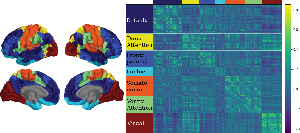
CN EMCI LMCI AD
3.10 Classifying Nodes
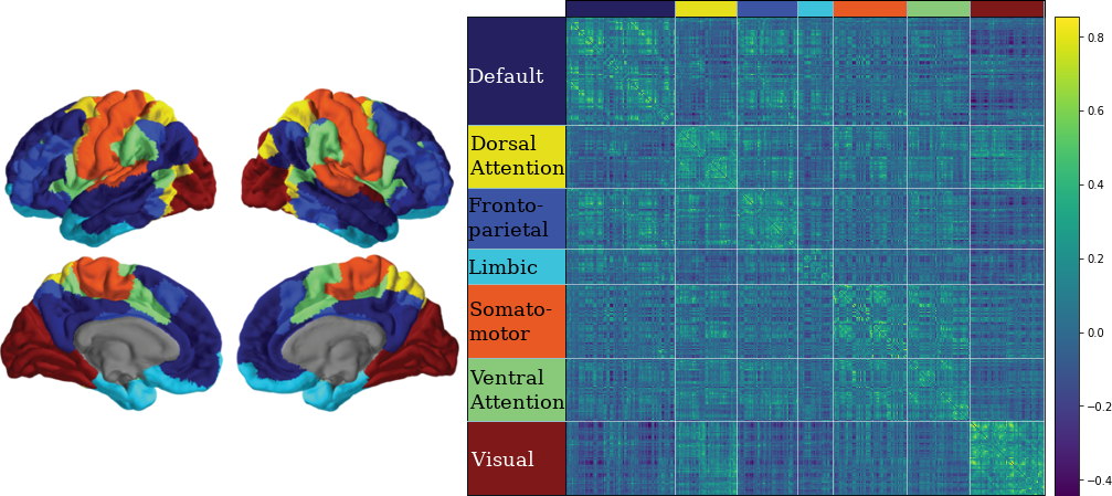
CN EMCI LMCI AD
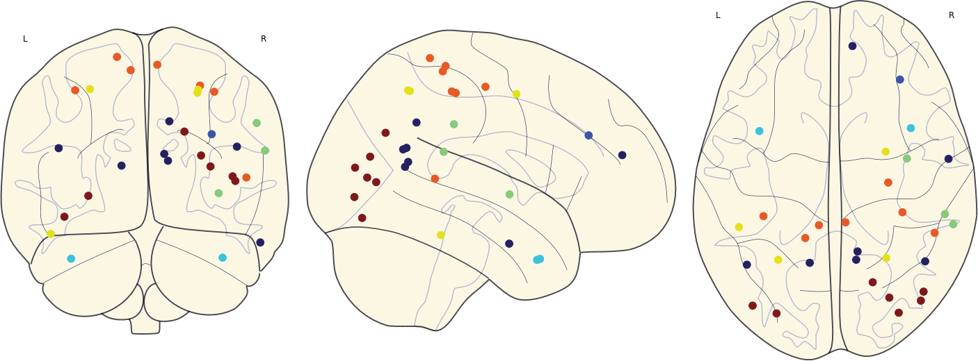
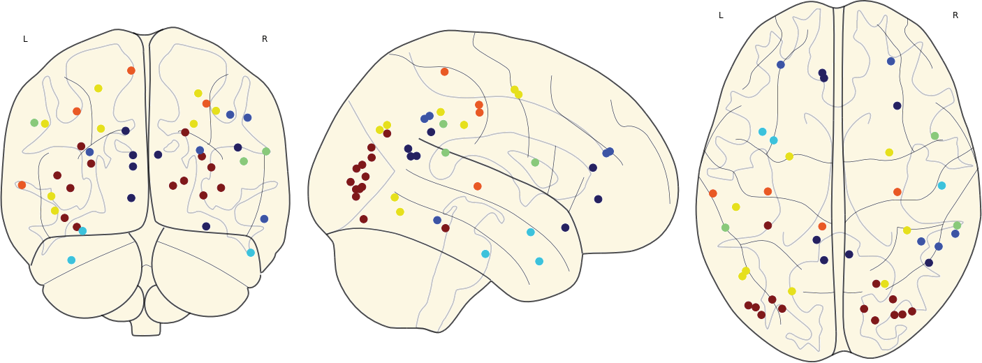
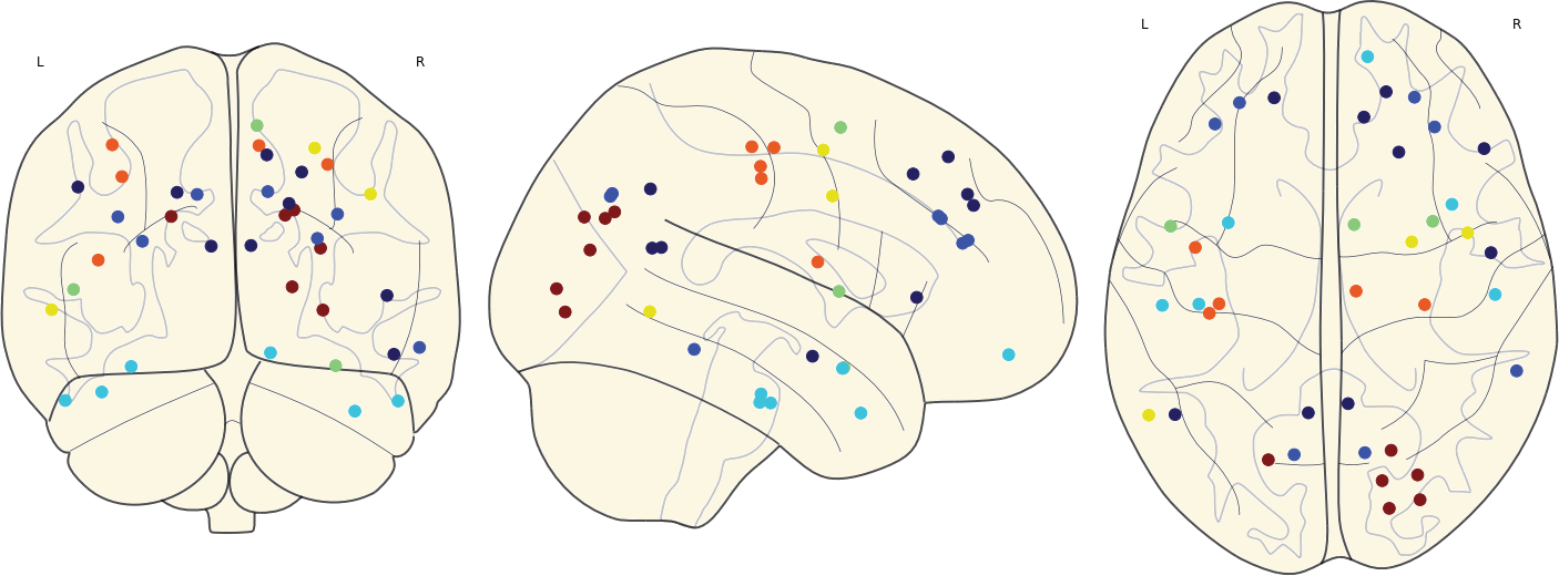
3.11 Hubs
Given a scoring system for nodes, network hubs are defined as nodes with score larger than the mean + the standard deviation of the scores of each node in the network.
Here we applied 3 different scores: Strength, Betweenness, and Clustering.
The network hubs are then the nodes which are hub based on one of these scores.
3.11 Hubs in the Mean Networks
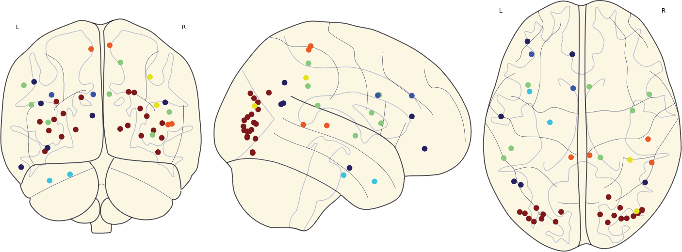
CN EMCI LMCI AD
3.11 Hubs in the Mean Networks

CN EMCI LMCI AD
3.11 Hubs in the Mean Networks

CN EMCI LMCI AD
3.11 Hubs in the Mean Networks

CN EMCI LMCI AD
3.11 Hubs in the Mean Networks
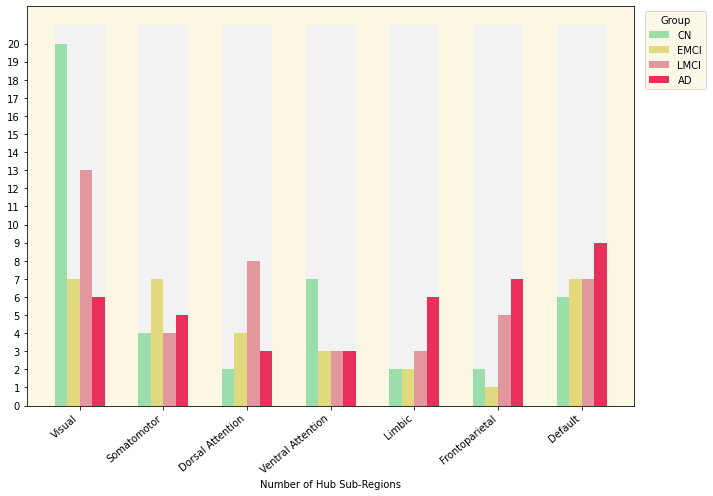
Group |
Number of Hubs |
|---|---|
| CN | 43 |
| EMCI | 31 |
| LMCI | 43 |
| AD | 39 |
3.12 Activated Links in Each Group
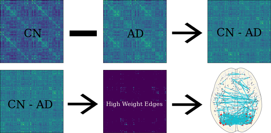
3.12 Activated Links in Each Group
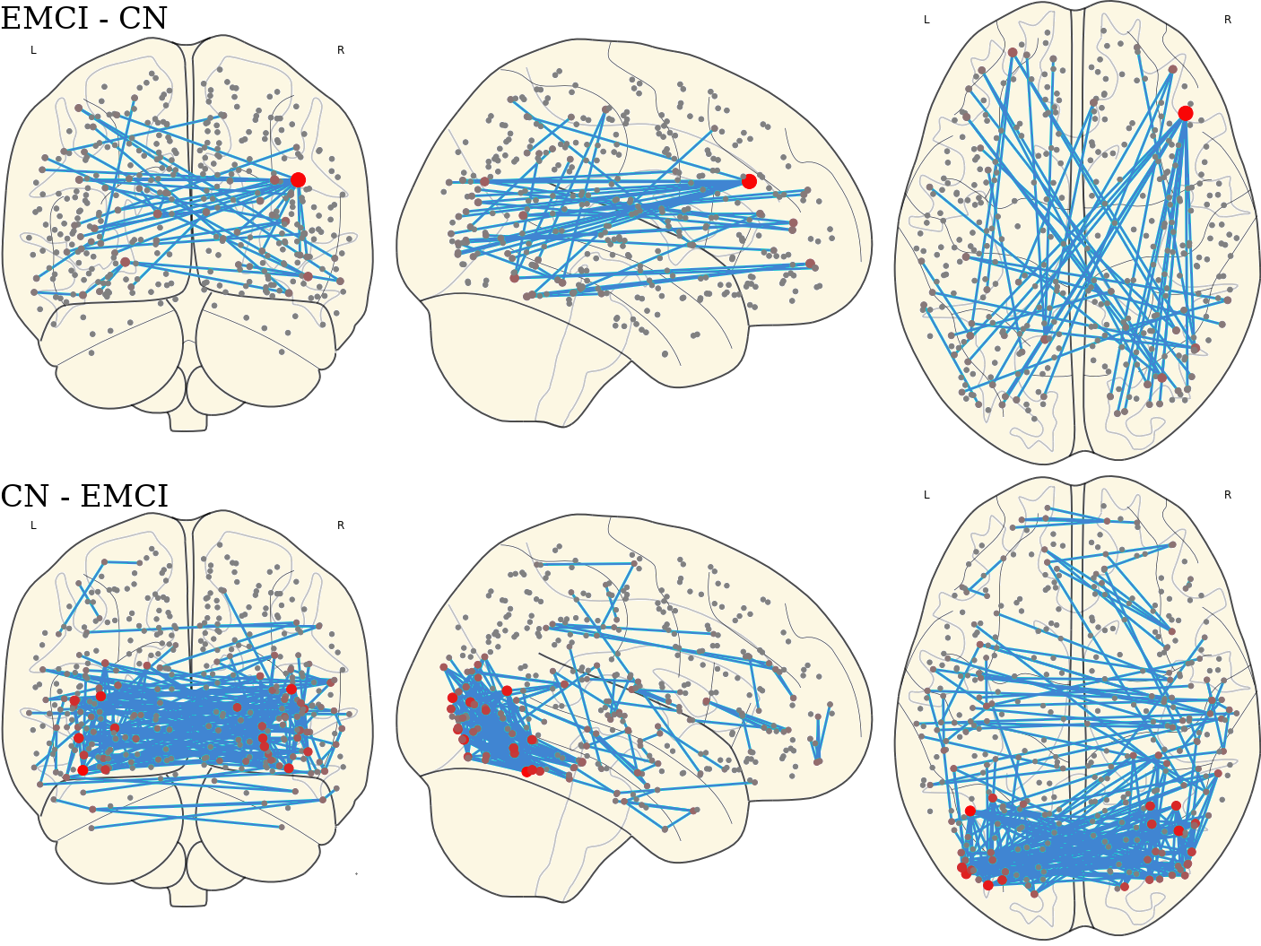
3.12 Activated Links in Each Group
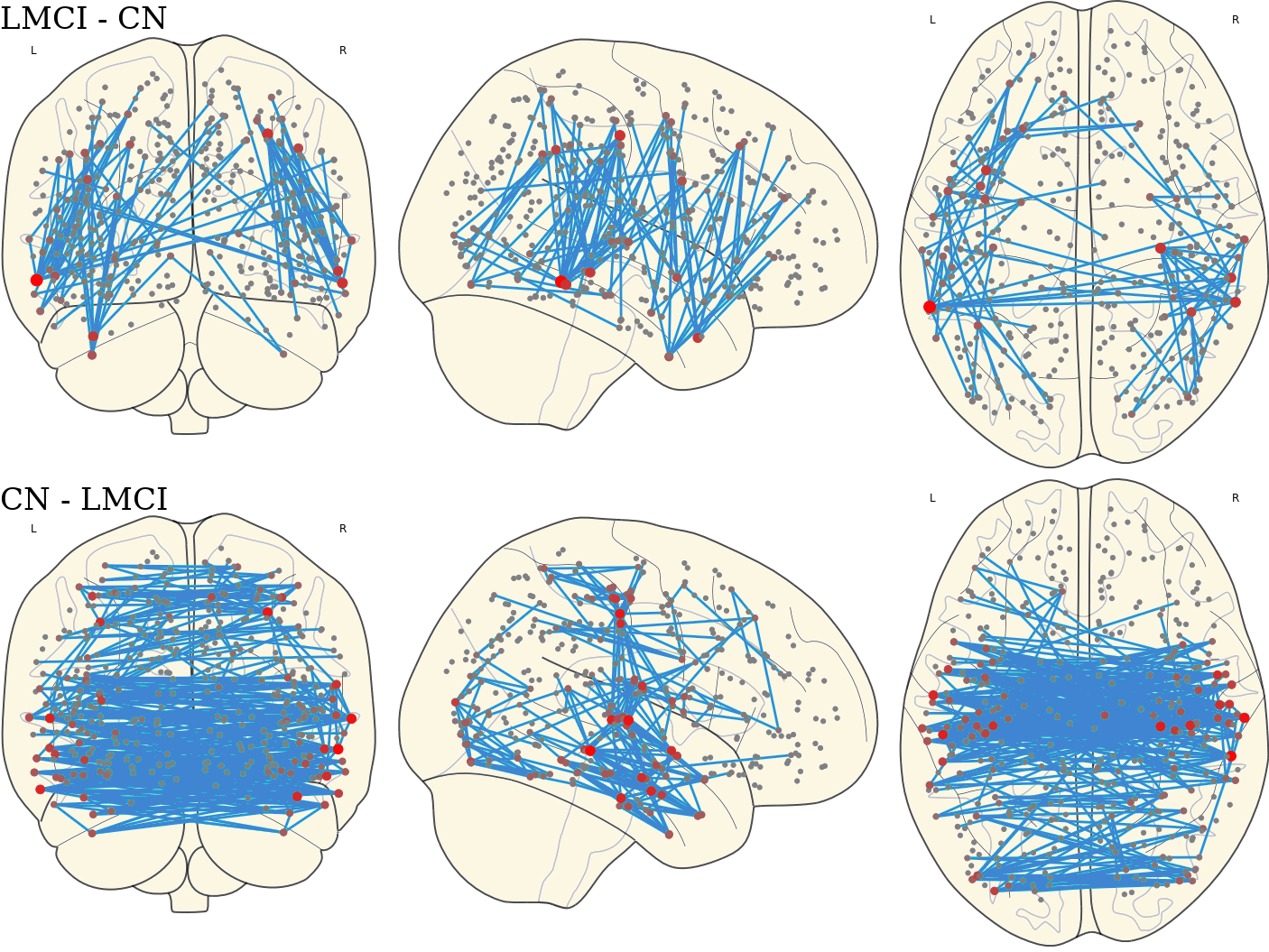
3.12 Activated Links in Each Group
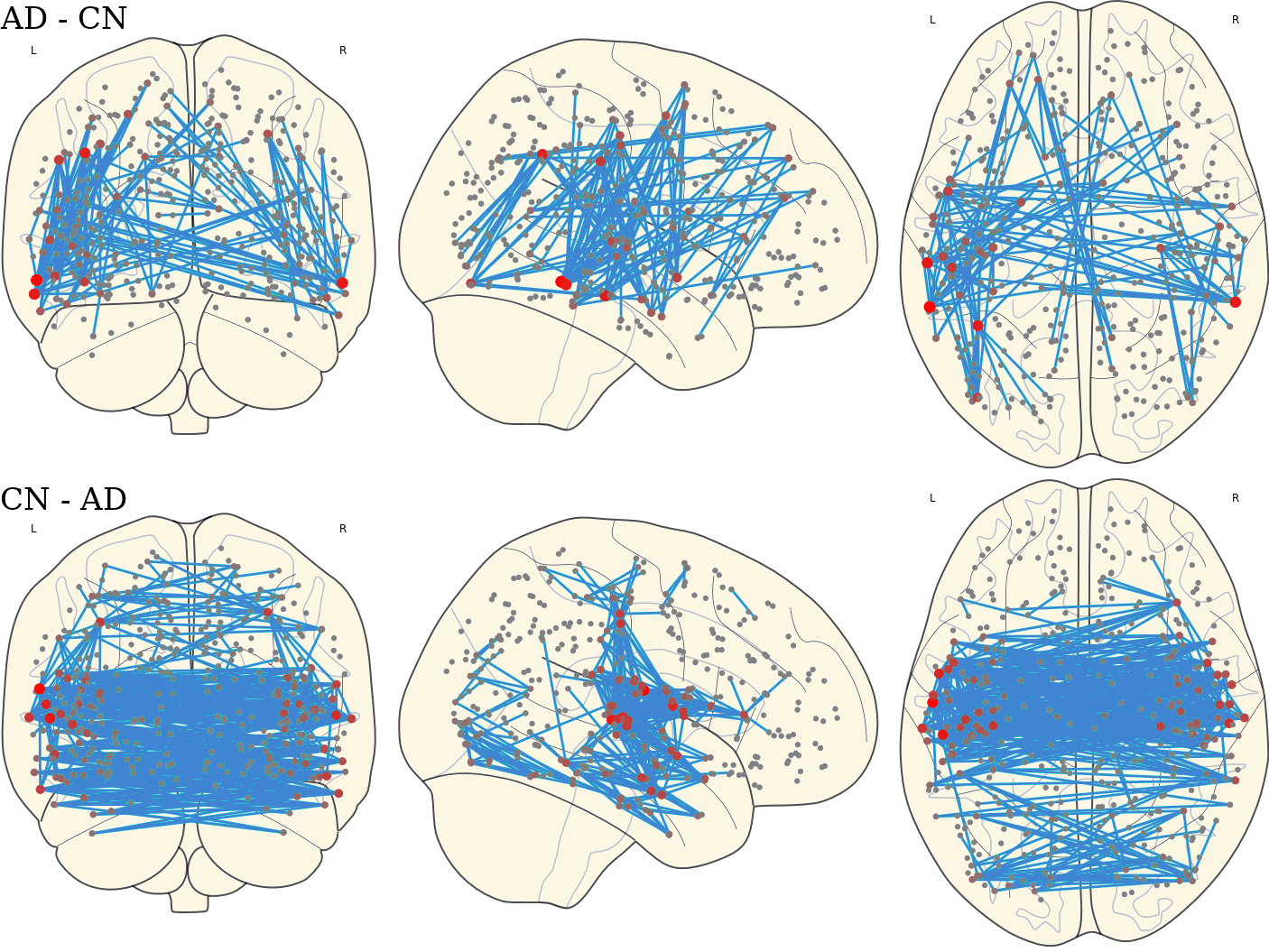
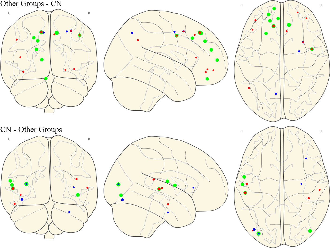
3.13 Activated ROIs in Each Group
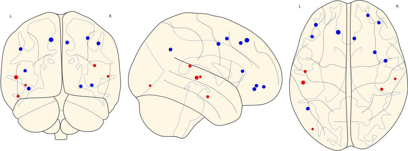
| CN | Other Groups |
3.13 Activated ROIs in Each Group
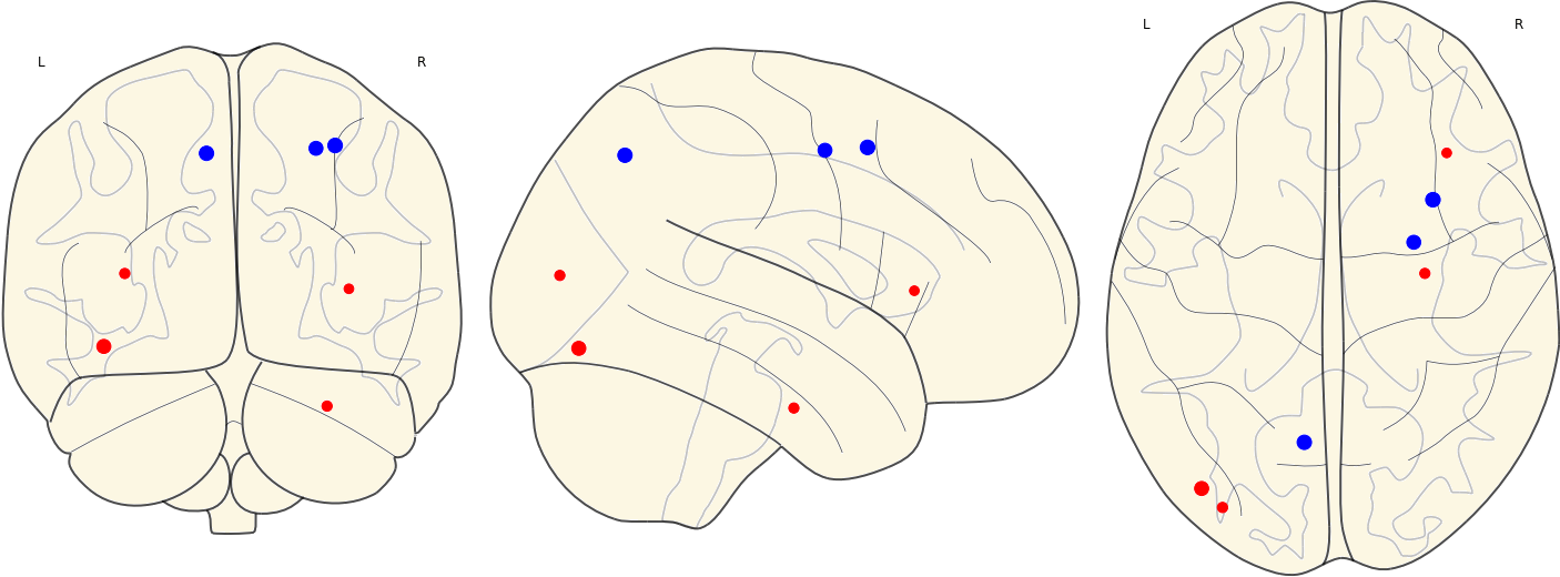
| CN | Other Groups |
3.13 Activated ROIs in Each Group
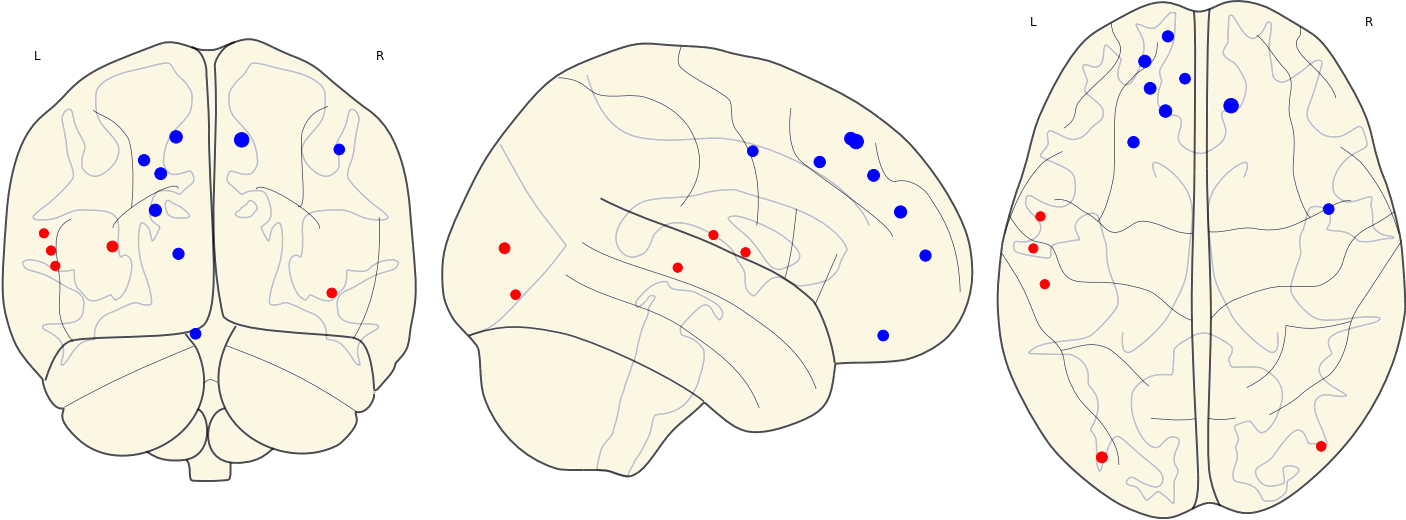
| CN | Other Groups |
3.13 Activated ROIs in Each Group
| EMCI |
| LMCI | AD |